Here I show how I designed a coaxial cavity bandpass filter. The method of Dishal is employed, using the k and q values. This was part of my Master’s Thesis, but here it is explained in more detail.

Design of such a filter is impossible without a 3D EM simulation software like CST, which is what I used for this project.

Cavity resonant frequency

First, we start with a single cavity. It has a side length of 25mm and a depth of 12mm. It is a coaxial cavity with a centre post having a diameter of 8mm.

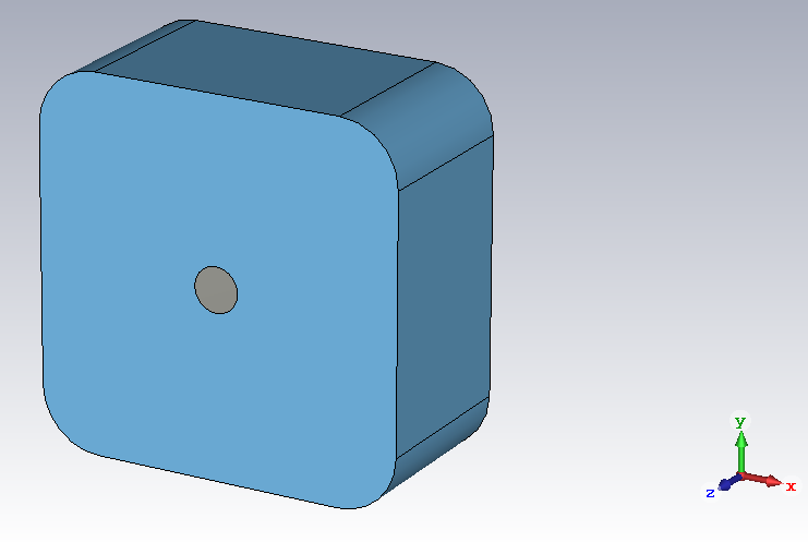
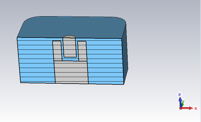
At the top cover, there is a tuning screw for frequency adjustment.

I want this filter to have a centre frequency of 2.5GHz. Therefore, I use the eigenmode solver to find the resonant frequency of the cavity as function of the tuning screw depth.

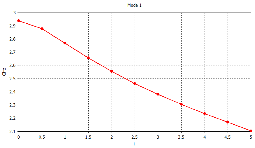
Using gnuplot or Matlab or another numeric software, I fit a function to these data points. The function used here is

\( f_0(t) = a_2\,t^2 + a_1\,t + a_0 \)

and it allows to precisely calculate the resonant frequency of the given cavity for any value of t, which is the tuning screw protrusion depth.

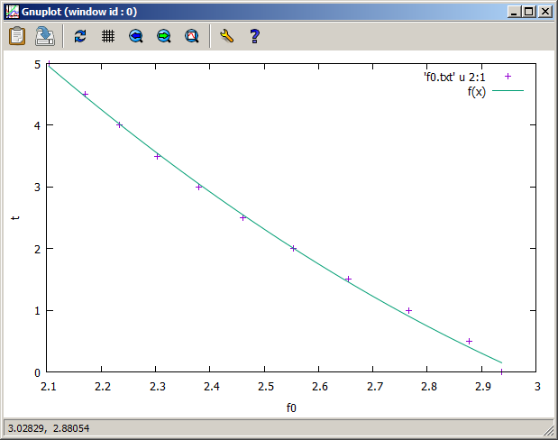
For a cavity having its resonant frequency at 2.5GHz, we easily find the tuning screw depth \( t = 2.315\,\text{mm} \).

Coupling between two cavities

The next step is to investigate the coupling between two adjacent cavities. For the filter to be designed, the cavities have a space between them of 2mm. There is a coupling iris, the width of which is adjusted.

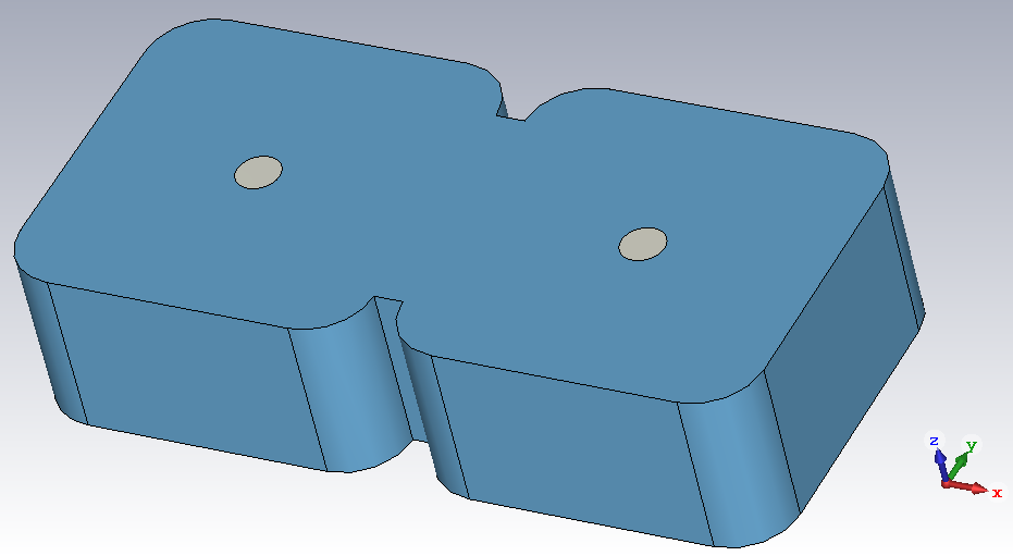
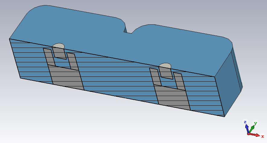
Since the tuning screw depth for a resonant frequency of 2.5GHz is known, this value is used now and both cavities are tuned to this same frequency. Next, we again use the eigenmode solver to find the first two resonant modes, which correspond to the even mode and to the odd mode, each of which having its own resonant frequency. One of them is slightly higher than 2.5GHz, the other is slightly lower than 2.5GHz. The iris width is adjusted and the resonant frequencies of the two modes are recorded. The coupling coefficient is then found as follows:

\( k = \frac{ f_2^2 – f_1^2 }{ f_2^2 + f_1^2 } \)

The coupling coefficient is calculated for 9 different iris widths:

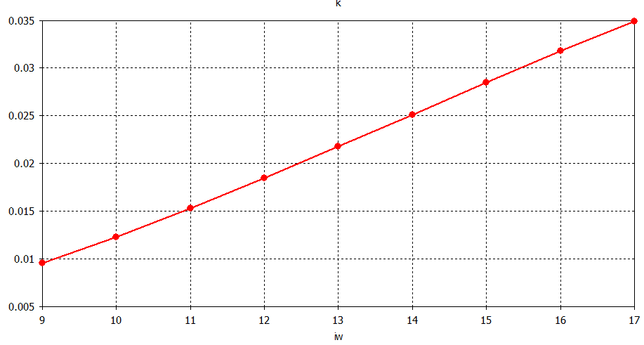
This data is then again processed by gnuplot and a function is fitted to it, such that the necessary iris width can easily be calculated if one knows the desired coupling coefficient.

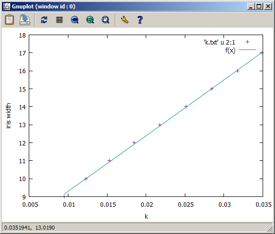
I used the function

\( w(k) = a\,\exp\left( b\,k \right) + c \)

because the function looks very linear, but it isn’t. The function now allows to find the necessary iris width for a given coupling coefficient. How cool is that? 🙂

Finding the external Q

Now one must also calculate the external quality factor of such a cavity. For this, I use the frequency domain solver. A cavity with two coaxial cables connected to it is simulated, as follows:

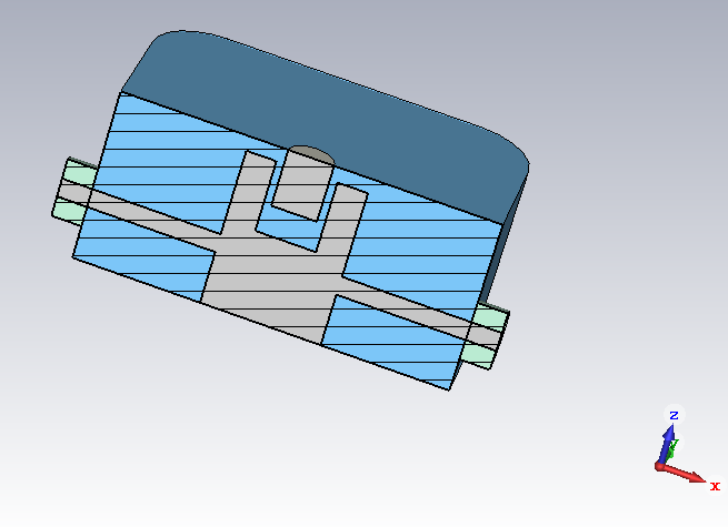
The frequency response of such a setup looks as follows:

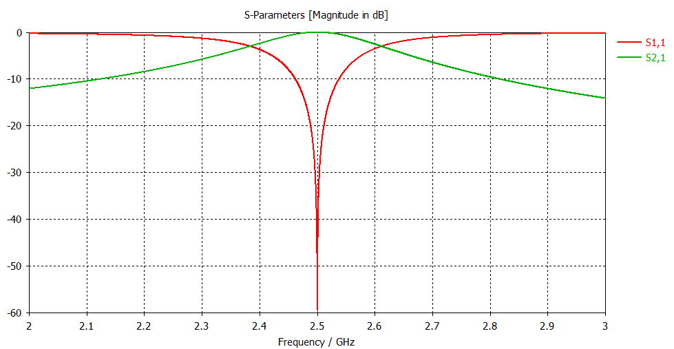
There is one resonance peak where \( S_{21} \) becomes 0dB. The peak has a bandwidth depending on the positions where the two coaxial cables are tapped at the centre post.

The external quality factor is found as follows:

\( Q_{ext} = \frac{ 2\,f_m }{ B } \)

where \( f_m \) is the peak frequency, and \( B \) is the 3dB bandwidth. The factor 2 is because the cavity is doubly loaded, i.e. there are 2 coaxial cables tapping the centre post, instead of only one.

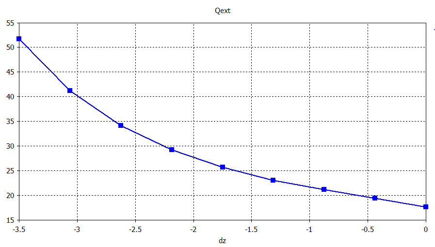
The frequency response is simulated for 9 different tap positions, and the external Q factor is recorded for each. The external Q will be higher and higher, the closer the tap comes to the lower end of the centre post. This gives following curve:

A gnuplot fit with the polynom

\( d_z(Q_{ext}) = a_3\,x^3 + a_2\,x^2 + a_1\,x + a_0 \)

yields the followig curve

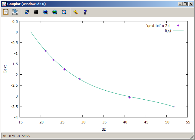
which is not perfect, but sufficient.

Designing the filter

With the equations published by Dishal, one can compute the necessary coupling coefficients and the external quality factor for a Butterworth or Chebyshev filter. I chose a Chebyshev filter with a ripple of 0.5dB, which gives the following coupling coefficients

\( \begin{gather}
k_{12} = 0.02631 \\
k_{23} = 0.02174 \\
k_{34} = 0.02119 \\
k_{45} = 0.02174 \\
k_{56} = 0.02631
\end{gather} \)

and an external Q of:

\(
Q_{ext} = 44
\)

Using the functions which i previously fitted in gnuplot, the iris widths can be calculated from the coupling coefficients, and the tap position is found from the external quality factor. This gives following dimensions:

\( \begin{gather}
w_{12} = 14.43 \\
w_{23} = 13.02 \\
w_{34} = 12.85 \\
w_{45} = 13.02 \\
w_{56} = 14.43 \\
d_z = -3.22
\end{gather} \)

Now, the initial design of the filter can be made, which gives the following geometry:

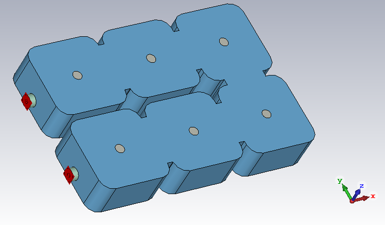
The Simulation of the initial design yields a quite distorted frequency response 🙁 this is because mainly the first and the last resonator are heavily detuned due to the tapping.

(TODO: insert missing graph of the initial frequency response. I did not yet dare to do so 🙂 )

After some tuning, I found a filter design which gives following frequency response:

Wow, that looks like the filter I would like to build. Then I made one…. milled out of a piece of aluminum! 😛

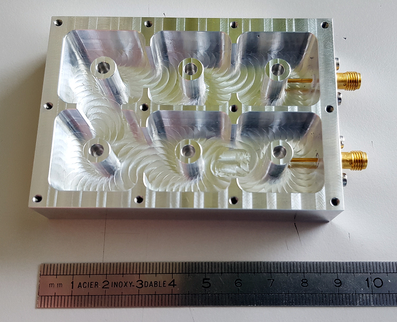
After manufacturing, the filter needs to be tuned using the tuning screws. The top cover looks like this from its bottom side:

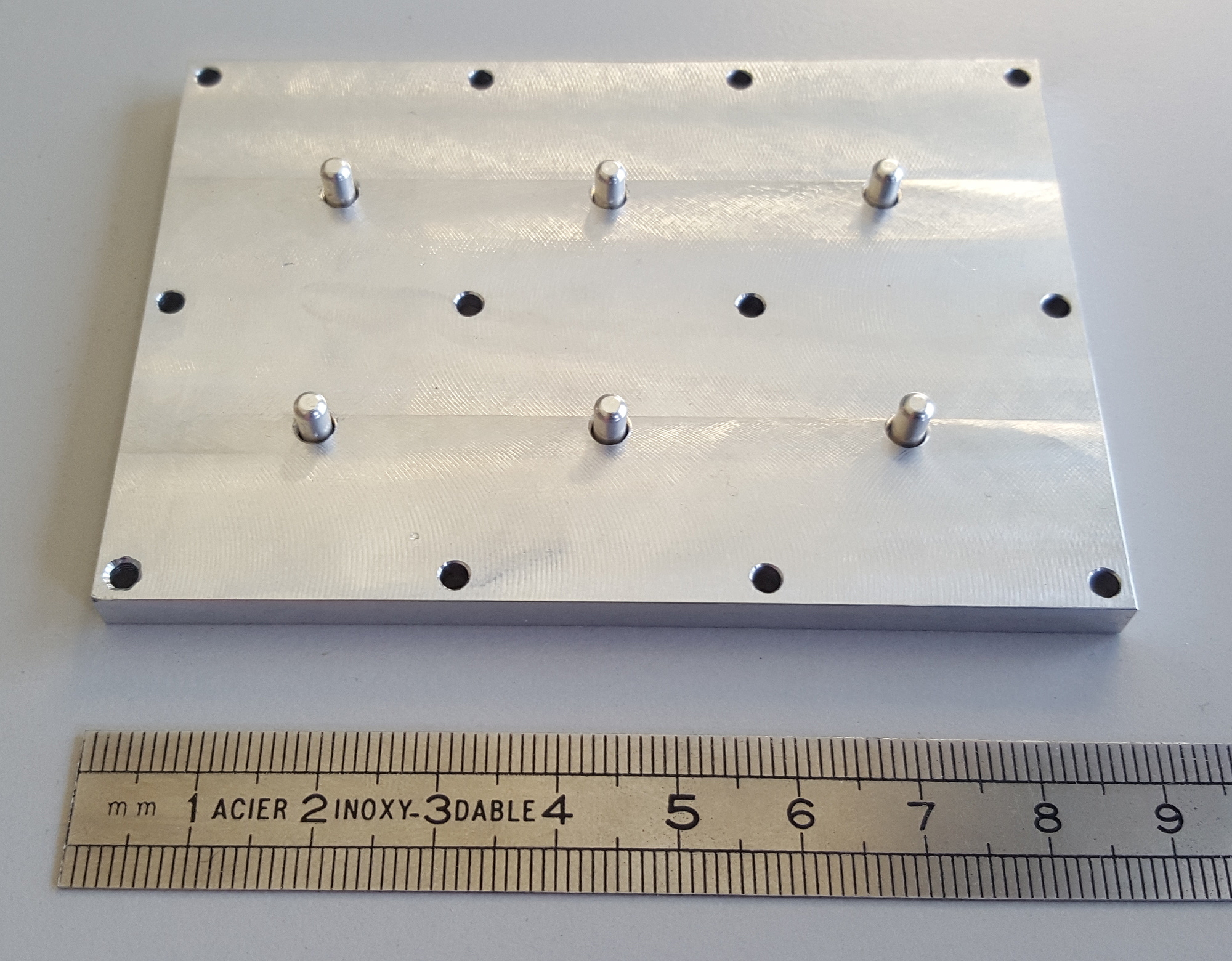
The little bumps are the bottom parts of the tuning screws. I used Dishal’s Method to tune the filter: heavily detune all resonators. Then measure Z11 using the network analyser, and tune the first resonator until Z11 is maximal. Then tune the next resonator until Z11 is minimal, and so on. This will yield the initial positions of the tuning screws. Afterwards, some fine-tuning can be applied. The result is quite nice:

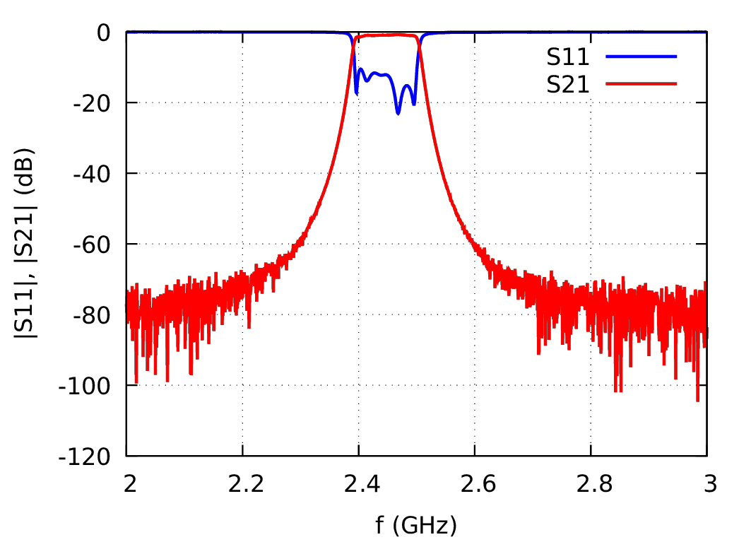
Note the 5 Dips in the S11 frequency response. Actually, there should be 6, one for each resonator. Apparently, the filter is still slightly mistuned. Further, there is also an insertion loss of about 0.5 dB. This is mainly due to the fact that the inner walls of the filter are not polished nor silver plated. Polishing has the largest effect and silver plating can be used if the last 0.01 dB are of a concern 🙂

I was wondering what properties this filter has concerning spurious pass-bands. Microstrip filters often have this kind of unwanted responses. When the coaxial resonators are analysed, one finds that the next higher eigenfrequency of a single resonator is around 11 GHz. So I would expect that at least one spurious passband occurs at 11 GHz…

… indeed there is! Cool fact: absolutely no spurious responses up to 11. Yay, finally I can tick that box on my bucket list:

[x] build a coaxial resonator filter

But today I read about “waffle iron filters” in the famous book “Microwave filters, impedance-matching networks, and coupling structures”. This yields a new box on my bucket list

Later, I will provide the final dimensions of the filter. I have it not at hand currently. My IEEE paper on that subject is still in progress…

Next time: an interesting microstrip lowpass filter!