Everybody knows that a matching network can be built using a quarterwave transformer. E.g. if a load of impedance \(Z_L\) shall be matched to a source having impedance \(Z_S\), this can be accomplished by using a transmission line with an electrical length of 90 degrees and characteristic impedance \(Z_0 = \sqrt{Z_S\,Z_L}\). However, is this also possible using lumped elements?
Yes it is! Remember that \(Z_0 = \sqrt{\frac{L}{C}}\). So, there are basically infinitely many combinations of \(L\) and \(C\) which give a desired characteristic impedance, but we can choose
\(C = \frac{1}{2\,\pi\,f_m\,Z_0}\)and
\(L = \frac{Z_0}{2\,\pi\,f_m}\).
This is shown in the following example. A load of 75 ohms needs to be matched to a source of 50 ohms at a centre frequency of 50 MHz. One finds \(Z_0 = 61.2\) and therefore \(C=52\,\mathrm{pF}\) and \(L=195\,\mathrm{nH}\). A quick simulation in LTSpice shows that indeed there is a good matching around 50 MHz:

The bandwidth with a return loss better than 30 dB is about 3 MHz, and the 20 dB return loss bandwidth is around 10 MHz.
Is it possible to increase the bandwidth? Yes! by cascading several of those matching networks. E.g. if one wants to match 50 to 75 ohms, it would be possible to match 50 to 62.5 ohms, and then 62.5 ohms to 75 ohms. I have done this in the following simulation:
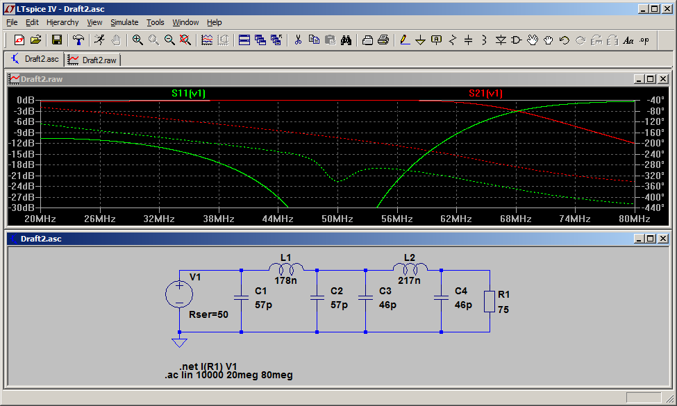
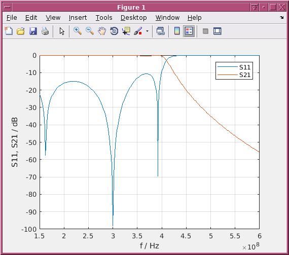
Note that this is like an arithmetic series, i.e. the difference between 50 ohms and 62.5 ohms is 12.5 ohms, and the difference between 62.5 and 75 ohms is also 12.5 ohms. If we had multiple intermediate stages, the difference would be always the same. For this above design, the bandwidth where the return loss is better than 30 dB is around 10 MHz, for 20 dB return loss it is around 16 MHz.
General network analysis
Consider the following network where the source and load impedances are labelled R1 and R2:
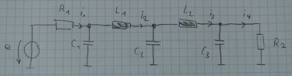
With the aid of the mesh rule (voltages around a loop add to zero), the currents in each of the loops can be found using the impedance matrix
$$ \mathbf{Z} \, \mathbf{I} = \mathbf{V} $$
with
$$ \mathbf{Z} =
\begin{pmatrix}
R_1 + \frac{1}{s\,C_1} & -\frac{1}{s\,C_1} & 0 & 0 \\
-\frac{1}{s\,C_1} & \frac{1}{s\,C_1} + s\,L_1 + \frac{1}{s\,C_2} & -\frac{1}{s\,C_2} & 0 \\
0 & -\frac{1}{s\,C_2} & \frac{1}{s\,C_2} + s\,L_2 + \frac{1}{s\,C_3} & -\frac{1}{s\,C_3} \\
0 & 0 & -\frac{1}{s\,C_3} & \frac{1}{s\,C_3} + R_2
\end{pmatrix}
$$
and:
$$
\mathbf{I} = \begin{pmatrix} I_1 \\ I_2 \\ I_3 \\ I_4 \end{pmatrix} \quad \mathbf{V}= \begin{pmatrix} e \\ 0 \\ 0 \\0 \end{pmatrix}
$$
To construct the impedance matrix for such ladded networks of arbitrary size, we can exploit the structure of the impedance matrix:
- the negative shunt impedances are on both off-diagonals
- the main diagonal contains the series impedances plus the shunt impedances
- the first and the last element also contain the two terminal impedances
With the Matlab script attached, matching networks of this type with arbitrary number of elements can be calculated and S11 and S21 are plotted as follows: